Product Sales Forecasting with Machine Learning

Introduction:
Effective sales forecasting is fundamental for multiple aspects of retail management and operation, including Inventory Management, Financial Planning, Marketing and Promotions, Supply Chain Optimization and Strategic Decision Making
In this blog, first we will perform EDA to understand the data and later we will explore how to build, optimize, and evaluate machine learning models to forecast sales amount and order volume.
Problem Statement:
In the competitive retail industry, the ability to predict future sales accurately is crucial for operational and strategic planning. Product sales forecasting aims to estimate the number of products a store will sell in the future, based on various influencing factors such as store type, location, regional characteristics, promotional activities, and temporal variations (such as holidays and seasons). This project focuses on developing a predictive model that uses historical sales data from different stores to forecast sales for upcoming periods.
Dataset Description:
Dataset contains 188340 unique transactions with 10 columns
1. ID: Unique identifier for each record in the dataset.
2. Store_id : Unique identifier for each store.
3. Store_Type : Categorization of the store based on its type.
4. Location_Type : Classification of the store’s location (e.g., urban, suburban).
5. Region_Code : Code representing the geographical region where the store is located.
6. Date : The specific date on which the data was recorded.
7. Holiday : Indicator of whether the date was a holiday (1: Yes, 0: No).
8. Discount : Indicates whether a discount was offered on the given date (Yes/No).
9. #Order : The number of orders received by the store on the specified day.
10. Sales : Total sales amount for the store on the given day.
Preprocessing:
When we read data as pandas DataFrame, it is good practice to convert column’s datatype such a way that data size can be optimal. Here, we have converted Store ID as unsigned-integer-16, Store Type, Location Type and Region Type as categorical, and Holiday and Discount as boolean to optimize the size of DataFrame and also make operations faster later on.
# Combine both the dataset into single dataframe
data = pd.concat([train, test])
data.reset_index(drop=True, inplace=True)

# Change Datatypes to optimize sizes
# Store_id as unsigned integer 16 (Range is 1 to 371)
data.Store_id = data.Store_id.astype('uint16')

# Store_Type, Location_Type, Region_Code as categorical
data.Store_Type = data.Store_Type.astype('category')
data.Location_Type = data.Location_Type.astype('category')
data.Region_Code = data.Region_Code.astype('category')

# Holiday and Discount as Boolean
data.Holiday = data.Holiday.astype('bool')
data.replace({'Discount':{'Yes':True, 'No':False}}, inplace=True)

# Drop unnecessary column Transaction ID
data.pop('ID')

# Set Date column as primary index
data.set_index('Date', inplace=True)
With this much datatype conversion size of data is reduced from 17.88 MB to 6.43 MB which is 64.04% reduction.
Feature Engineering:
Developing correct features helps us to understand data better and train more accurately. Features like Year, QUarter, Month, MonthName, Week, Day, DayNamenetc are developed from date column.
data['Year'] = data.index.year
data['Quarter'] = data.index.quarter
data['Month'] = data.index.month
data['MonthName'] = data.index.month_name()
data['Day'] = data.index.day
data['Week'] = data.index.isocalendar().week
data['Weekday'] = data.index.weekday
data['DayName'] = data.index.day_name()
data['Weekend'] = data.Weekday.apply(lambda x: 'Weekend' if x in ['Saturday','Sunday'] else 'Weekday')
EDA:
Visualization dashboard is developed using tableau can be found here https://public.tableau.com/app/profile/mathrunner7/viz/ProductSalesForecasting_17346981632090/TimeseriesDashboard
Here, we will focus more in visualization using python and plotly package.
Univariate Analysis:
Histogram plots are great to observe distribution of data visually. From the plot below we can conclude that data is almost normally distributed with outliers present.
fig = make_subplots(rows=1, cols=3,
                    subplot_titles=('Order','Sales','Sales per Order'))
fig.add_trace(go.Histogram(x=train.Order), row=1, col=1)
fig.add_trace(go.Histogram(x=train.Sales), row=1, col=2)
fig.add_trace(go.Histogram(x=train['S/O']), row=1, col=3)
fig.update_layout(title='Distribution of target parameters',
                  showlegend=False, title_x=0.5, title_y=0.1)
fig.show()
Top & Bottom Store IDs:
Aggregating data by Store IDs and visualizing it gives us best and worst performing stores. Despite Order volume and Sales amount are having high positive correlation, some stores are not in top/bottom 10 of sales and order both together.
fig = make_subplots(rows=2, cols=1, subplot_titles=('Top/Bottom 10 Store IDs', ''))
top_order = train.groupby('Store_id').agg({'Order':'sum'}).sort_values('Order', ascending=False).head(10)
top_sales = train.groupby('Store_id').agg({'Sales':'sum'}).sort_values('Sales', ascending=False).head(10)
bottom_order = train.groupby('Store_id').agg({'Order':'sum'}).sort_values('Order', ascending=False).tail(10)
bottom_sales = train.groupby('Store_id').agg({'Sales':'sum'}).sort_values('Sales', ascending=False).tail(10)
tb_order = pd.concat([top_order, bottom_order])
tb_sales = pd.concat([top_sales, bottom_sales])
fig.add_trace(go.Bar(x=tb_order.index, y=tb_order.Order, name='Order', marker=dict(color=order_color)), row=1, col=1)
fig.add_trace(go.Bar(x=tb_sales.index, y=tb_sales.Sales, name='Sales', marker=dict(color=sales_color)), row=2, col=1)
fig.update_layout(xaxis=dict(type='category'),
                  xaxis2=dict(type='category'),
                  yaxis=dict(title='Order Volume'),
                  yaxis2=dict(title='Sales Amount'),
                  showlegend=False)
fig.show()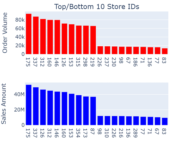
Bivariate Analysis:
Bar charts in grid is one of the simplest and easiest way to visualize and compare categorical distributions. From bar charts we can identify Store Type S1 & S4 are having higher sells compared to S2 & S3. Location L4 & L5 are having negligible amount of sales. And in region majority of business is coming from R1 followed by R2m R3 & R4. Weekends have slight higher sales compared to weekdays.
order_color = 'red'
sales_color = 'blue'
fig = make_subplots(rows=2, cols=4)
grouped = train.groupby('Store_Type').agg({'Order':'sum','Sales':'sum'})
fig.add_trace(go.Bar(x=grouped.index, y=grouped.Order, marker=dict(color=order_color)), row=1, col=1)
fig.add_trace(go.Bar(x=grouped.index, y=grouped.Sales, marker=dict(color=sales_color)), row=2, col=1)
grouped = train.groupby('Location_Type').agg({'Order':'sum','Sales':'sum'})
fig.add_trace(go.Bar(x=grouped.index, y=grouped.Order, marker=dict(color=order_color)), row=1, col=2)
fig.add_trace(go.Bar(x=grouped.index, y=grouped.Sales, marker=dict(color=sales_color)), row=2, col=2)
grouped = train.groupby('Region_Code').agg({'Order':'sum','Sales':'sum'})
fig.add_trace(go.Bar(x=grouped.index, y=grouped.Order, marker=dict(color=order_color)), row=1, col=3)
fig.add_trace(go.Bar(x=grouped.index, y=grouped.Sales, marker=dict(color=sales_color)), row=2, col=3)
grouped = train.groupby(['Weekday','DayName']).agg({'Order':'sum','Sales':'sum'}).reset_index()
fig.add_trace(go.Bar(x=grouped.DayName, y=grouped.Order, marker=dict(color=order_color)), row=1, col=4)
fig.add_trace(go.Bar(x=grouped.DayName, y=grouped.Sales, marker=dict(color=sales_color)), row=2, col=4)
fig.update_layout(title='Order, Sales and Sales/Order distribution', showlegend=False, title_x=0.5, title_y=0.85)

fig.update_yaxes(title='Order Volume', row=1, col=1)
fig.update_yaxes(title='Sales Amount', row=2, col=1)

fig.update_xaxes(title='Store Type', row=2, col=1)
fig.update_xaxes(title='Location Type', row=2, col=2)
fig.update_xaxes(title='Region Code', row=2, col=3)

fig.show()
Scatter Plots:
Scatter plot gives us idea about how two variables are correlated to each other for a given category.
def scatter_plots(df, column):
  categories = df[column].astype('category').unique().sort_values()
  fig = make_subplots(rows=1, cols=len(categories),
                      subplot_titles=[str(c) for c in categories])
  for i, category in enumerate(categories):
    fig.add_trace(go.Scatter(x=df[df[column] == category]['Order'],
                             y=df[df[column] == category]['Sales'],
                             mode='markers', marker=dict(size=2), name=category,),row=1, col=i+1)
    fig.update_xaxes(range = [0,300], row=1, col=i+1)
    fig.update_yaxes(range = [0,250000], row=1, col=i+1)
  fig.update_layout(title=f'{column} wise Order v/s Sales Scatter Plot', height = 400, showlegend=False, title_x=0.5)
  fig.show()
Here all the scatter plot indicates that Order volume and Sales amount have strong positive correlation. However if we compare scatter plots with bar charts above, it is evident that despite S1 and S3 store types have similar range of order volume and sales amount, S1 has higher cumulative sales which means number of transactions are high for S1 compared to S3. Same conclusion can be made for locations also, where L1 having highest cumulative sales doesn’t have high order count or sales amount , but has more number of transactions compared to L2.


Holiday scatter plot tells us that when there is holiday transaction density is high but high sales value transactions can be found during working days.
Same goes for Discount, where discount days encourages people to spend more compared to regular transaction days.


Hypothesis Testing:
Hypothesis testing gives us statistical proof with certain confidence about our assumption on the data.
χ² test:
Following code performs χ² test for given category combinations and returns if the two categories are dependent on each other or not.
Null Hypothesis H0 = Categories are independent of each other
Alternate Hypothesis H1 = Categories are dependent
from scipy.stats import chi2_contingency

def chi2test(data, category1, category2, alpha=0.05):
  data = data.groupby(by=[category1, category2]).agg({'Order':'sum', 'Sales':'sum'}).reset_index()
  test = chi2_contingency(data.pivot(index=category1,columns=category2,values='Order').fillna(0))
  order_dependency = test.pvalue < alpha
  if order_dependency:
    print(f'Reject the Null Hypothesis. For Order volume, {category1} and {category2} are dependent', end=" | ")
  else:
    print(f'Fail to reject the Null Hypothesis. For Order volume, {category1} and {category2} are independent', end=" | ")
  print(f'Test statistics:{test.statistic},\tp-value:{test.pvalue}')

  test = chi2_contingency(data.pivot(index=category1,columns=category2,values='Sales').fillna(0))
  sales_dependency = test.pvalue < alpha
  if sales_dependency:
    print(f'Reject the Null Hypothesis. For Sales amount, {category1} and {category2} are dependent', end=" | ")
  else:
    print(f'Fail to reject the Null Hypothesis. For Sales amount, {category1} and {category2} are independent', end=" | ")
  print(f'Test statistics:{test.statistic},\tp-value:{test.pvalue}')

  return {'C1':category1, 'C2':category2,'Order': order_dependency, 'Sales': sales_dependency}

# Perform Chi-Squared test for category combinations
columns = ['Store_Type', 'Location_Type', 'Region_Code', 'Holiday', 'Discount', 'MonthName', 'DayName']
dependancy_summary = pd.DataFrame([chi2test(train,c1,c2) for c1,c2 in list(permutations(columns,2))])
Result of the χ² test is converted into dependency table where True means that category pair is dependent.

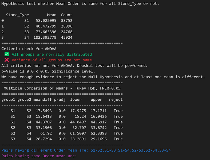
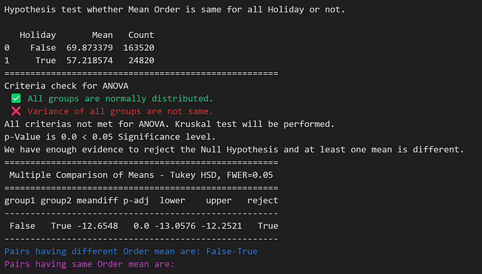
Mean Similarity Test:
Following code performs mean similarity test. If performs ANOVA if data satisfy assumptions for it otherwise performs TukeyHSD to check is all categories have same mean or not. It also returns list of pairs having same mean and different mean.
Null Hypothesis H0 = All categories have same mean
Alternate Hypothesis H1 = There is atleast once category having different mean
from scipy.stats import f_oneway, kruskal, anderson, levene
from statsmodels.stats.multicomp import pairwise_tukeyhsd
from itertools import combinations

def decorator(func):
  def wrapper(*args, **kwargs):
    print('~'*100)
    print('~'*100)
    result = func(*args, **kwargs)
    print('~'*100)
    print('~'*100)
    return result
  return wrapper

@decorator
def variance_test(data, category, target, alpha=0.05):
  d = data.groupby(by=category).agg(Mean=(target,'mean'), Count=(target, 'size')).reset_index()
  print(f'Hypothesis test whether Mean {target} is same for all {category} or not.\n')
  print(d)
  print('='*53)
  cats = sorted(data[category].unique())
  groups = {}
  for cat in cats:
     groups[cat]=data[data[category] == cat][target]

  # Check for Normality test of all categories
  normality_test = True
  print('Criteria check for ANOVA')
  for cat,group in groups.items():
    if not anderson(group).fit_result.success:
      normality_test = False
      print(f'\033[31m \u274C Group {cat} is not normally distributed.\033[0m')
      break
  if normality_test:
    print('\033[32m \u2705 All groups are normally distributed.\033[0m')
  # Check for levene test
  levene_test = True
  _, p_levene = levene(*groups.values())
  if p_levene < alpha:
    levene_test = False
    print(f'\033[31m \u274C Variance of all groups are not same.\033[0m')
  else:
    print(f'\033[32m \u2705 Variance of all groups are same.\033[0m')

  # Perform One-way ANOVA if criteria meets otheriwse perform Kruskal
  if normality_test and levene_test:
    print('One-Way ANOVA will be performed.')
    _, p_value = f_oneway(*groups.values())
  else:
    print('All criterias not met for ANOVA. Kruskal test will be performed.')
    _, p_value = kruskal(*groups.values())

  # Proceed for ttest_ind if one group has different mean
  if p_value > alpha:
    print(f'p-Value is {p_value} > {alpha} Significance level.\nWe dont have enough evidence to  reject the Null Hypothesis. All means are same.')
    print('='*53)
    return None
  else:
    print(f'p-Value is {p_value} < {alpha} Significance level.\nWe have enough evidence to reject the Null Hypothesis and at least one mean is different.')
    print('='*53)

  tukey = pairwise_tukeyhsd(endog=data[target], groups=data[category], alpha=0.05)
  print(tukey)
  # Extract group1 and group2 using the Tukey object attributes
  group1 = tukey.groupsunique[tukey._multicomp.pairindices[0]]
  group2 = tukey.groupsunique[tukey._multicomp.pairindices[1]]
  pair = [f'{a}-{b}' for a,b in list(zip(group1, group2))]
  reject = tukey.reject

  # Combine group1 and group2 into a DataFrame
  group_pairs = pd.DataFrame({'pair': pair, 'reject': reject})
  same_mean_pairs = group_pairs[group_pairs['reject'] == False]['pair']
  different_mean_pairs = group_pairs[group_pairs['reject'] == True]['pair']
  print(f'\033[34mPairs having different {target} mean are: {",".join(different_mean_pairs.values)}')
  print(f'\033[35mPairs having same {target} mean are: {",".join(same_mean_pairs.values)}\033[0m')

  return None
Two such examples are shown below.
Data Preparation for Model Building:
To prepare the data for model building we have considered aggregation and table transformation using pandas standard pd.crosstab() method and then join all the tables on date index to have one single table which can be used to train the models. We are going to use SARIMAX family of algorithms from statsmodels package to train our forecasting model.
# Data Preperation for modeling
# Data for Sales forecastig model training
overall_sales = train.groupby(level=0).agg({'Sales':'sum'})
id_wise_sales = pd.crosstab(index=train.index, columns=train.Store_id, values =train.Sales, aggfunc='sum')
store_type_wise_sales = pd.crosstab(index=train.index, columns=train.Store_Type, values =train.Sales, aggfunc='sum')
location_wise_sales = pd.crosstab(index=train.index, columns=train.Location_Type, values =train.Sales, aggfunc='sum')
region_wise_sales = pd.crosstab(index=train.index, columns=train.Region_Code, values =train.Sales, aggfunc='sum')
# Data for Order forecastig model training
overall_order = train.groupby(level=0).agg({'Order':'sum'})
id_wise_order = pd.crosstab(index=train.index, columns=train.Store_id, values =train.Order, aggfunc='sum')
store_type_wise_order = pd.crosstab(index=train.index, columns=train.Store_Type, values =train.Order, aggfunc='sum')
location_wise_order = pd.crosstab(index=train.index, columns=train.Location_Type, values =train.Order, aggfunc='sum')
region_wise_order = pd.crosstab(index=train.index, columns=train.Region_Code, values =train.Order, aggfunc='sum')
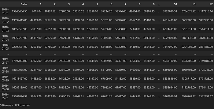
# Create a Single DataFrame for Sales and Order
train_sales = pd.concat([overall_sales, id_wise_sales, store_type_wise_sales, location_wise_sales, region_wise_sales], axis=1)
train_order = pd.concat([overall_order, id_wise_order, store_type_wise_order, location_wise_order, region_wise_order], axis=1)
exog_train_holiday = train.groupby(train.index).mean('Holiday')['Holiday']
exog_test_holiday = test.groupby(test.index).mean('Holiday')['Holiday']Final table looks like this and here each column will be trained separately.
Stationarity check and Correlation charts:
Before proceeding to model building knowing about stationarity of the data and ACF/PACF chart can give us good idea about hyperparameter selection.
Dickey-Fuller Test:
Dickey-fuller test is statistical method to check whether data is stationary or not. Following code snippet performs augmented dickey-fuller test and prints if the timeseries is stationary or not.
def adf_test(dataset):
  print(f'Results of Dickey-Fuller Test:')
  for column in dataset.columns:
    pvalue = adfuller(dataset[column])[1]
    if pvalue <= 0.05:
      print(f'\033[32mTimeseries for "{column}" is stationary', end='.\t')
    else:
      print(f'\033[31mTimeseries for "{column}" is not stationary', end='.')
    print(f'\tp-value is {pvalue}\033[0m')
ACF/PACF Chart:
We can find probable values of hyperparameter “p” and “q” from ACF and PACF charts. Cut-off point in PACF gives us basic idea about auto regression order p, whereas cut-off point in ACF gives idea about moving average order q. Looking from ACF/PACF charts for all proposed timeseries we can conclude that “p” is 1 and “q” can be either 1 or 2.
def acf_pacf_plot(series_sales:pd.Series,series_order:pd.Series)->None:
  fig, (ax1, ax2, ax3, ax4) = plt.subplots(1, 4, figsize=(14, 5))
  # Plot Sales ACF in first cell
  plot_acf(series_sales, ax=ax1)
  ax1.set_title(f'ACF for {series_sales.name} Sales')
  # Plot Sales PACF in second cell
  plot_pacf(series_sales, ax=ax2)
  ax2.set_title(f'PACF for {series_sales.name} Sales')

  # Plot Sales ACF in first cell
  plot_acf(series_order, ax=ax3)
  ax3.set_title(f'ACF for {series_sales.name} Order')
  # Plot Sales PACF in second cell
  plot_pacf(series_order, ax=ax4)
  ax4.set_title(f'PACF for {series_sales.name} Order')

  # Adjust layout
  plt.tight_layout()
  plt.show()

acf_pacf_plot(train_sales["R1"], train_order["R1"])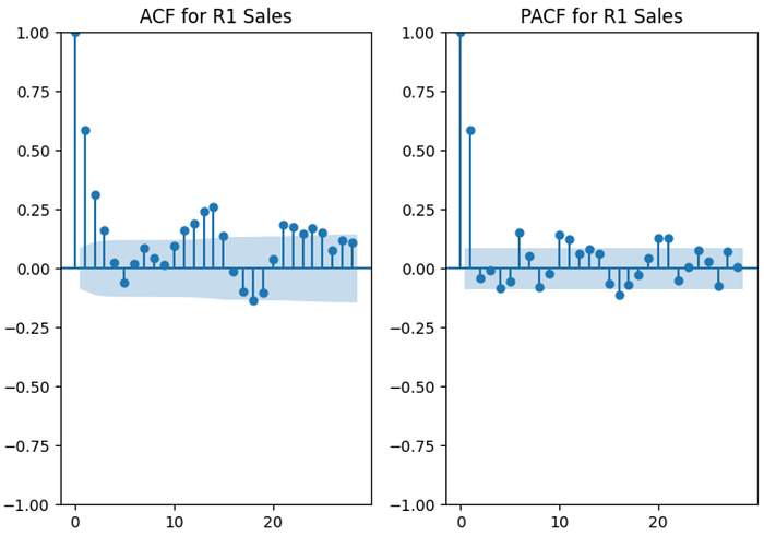
Seasonality:
Seasonality chart can be generated using following code after decomposing the model. It gives us idea about seasonal parameter “S” in model training.
from statsmodels.tsa.seasonal import seasonal_decompose

def seasonal_chart(series_sales, series_order):

  fig, (ax1, ax2) = plt.subplots(1, 2, figsize=(14, 5))
  # Plot Sales Seasonality in first cell
  result = seasonal_decompose(series_sales, model='additive', period=None)
  result.seasonal.plot(ax=ax1)
  ax1.set_title(f'Seasonality for {series_sales.name} Sales')
  # Plot Order Seasonality in second cell
  result = seasonal_decompose(series_order, model='additive', period=None)
  result.seasonal.plot(ax=ax2)
  ax2.set_title(f'Seasonality for {series_order.name} Order')

  # Adjust layout
  plt.tight_layout()
  plt.show()

seasonal_chart(train_sales["L3"], train_order["L3"])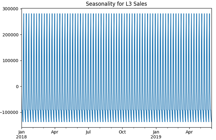
Train-test split:
In timeseries we cannot split data randomly for train and test operations. Out of all date wise sorted rows we need to consider first 80% (or whatever proportion we decide) data as train and tailing 20% data as test. Instead of doing this activity manually everytime we can define a class which will perform splitting data into requored porportion with single line command.
from sklearn.base import BaseEstimator, TransformerMixin

class TimeSeriesSplitter(BaseEstimator, TransformerMixin):
    def __init__(self, test_size=0.2):
        self.test_size = test_size
        self.train_data, self.test_data = None, None

    def fit(self, X, y=None):
        """No fitting required; just for compatibility."""
        return self

    def transform(self, X, y=None):
        """Split the single-column time series into train and test sets."""
        n_rows = len(X)
        split_index = int(n_rows * (1 - self.test_size))
        self.train_data = X.iloc[:split_index].asfreq('D')
        self.test_data = X.iloc[split_index:].asfreq('D')
        return self.train_data, self.test_data
Model Training:
Model training is most crucial stage in time series forecasting. As SARIMAX is not standard scikit-learn algorithm family, we have developed child class which will perform operations like fit, predict and score.
from statsmodels.tsa.statespace.sarimax import SARIMAX
from sklearn.base import BaseEstimator
from sklearn.metrics import (make_scorer, mean_squared_error as mse, mean_absolute_error as mae, mean_absolute_percentage_error as mape)

class SARIMAXEstimator(BaseEstimator):
    def __init__(self, order=(1,0,1), seasonal_order = (1,0,1,12)):
        self.order = order
        self.seasonal_order = seasonal_order
        self.model_ = None

    def fit(self, X, exog=None):
      self.exog_train=exog
      try:
        if isinstance(self.exog_train, pd.Series):
          self.model_ = SARIMAX(X, exog=self.exog_train, order=self.order, seasonal_order=self.seasonal_order).fit(disp=False)
        else:
          self.model_ = SARIMAX(X, order=self.order, seasonal_order=self.seasonal_order).fit(disp=False)
      except Exception as e:
        print(f"Skipping: order={self.order}, seasonal_order={self.seasonal_order}. Error: {e}")
        self.model_ = None
      return self

    def predict(self, n_steps, exog=None):
      if self.model_ is None:
        return np.full(n_steps, 1E-10)
      try:
        if not isinstance(self.exog_train, pd.Series):
          return self.model_.forecast(steps=n_steps)
        elif isinstance(exog, pd.Series):
          return self.model_.forecast(steps=n_steps, exog=exog[:n_steps])
        else:
          raise ValueError('No exog data provided')
      except Exception as e:
        print(e)
      return None

    def score(self, X, exog=None):
        n_steps = len(X)
        predictions = self.predict(n_steps, exog)
        return mape(X, predictions)
Multiple train run with ML Flow and Model selection:
With the help of MLFlow package we can do experiment tracking which helps use to save time and avoids repetition of same job.
mlflow.set_experiment("Sore ID Sales Forecasting-1.1.0")
for column in train_sales.columns:
  splitter = TimeSeriesSplitter()
  X_train, X_test = splitter.fit_transform(train_sales[column])
  X_train_exog, X_test_exog = splitter.fit_transform(exog_train_holiday)
  for order, seasonal in param_grid:
    with mlflow.start_run():
      sarimax_estimator = SARIMAXEstimator(order=order, seasonal_order=seasonal)
      sarimax_estimator.fit(X=X_train, exog=X_train_exog)
      model_score = sarimax_estimator.score(X=X_test, exog=X_test_exog)
      mlflow.set_tag('data', column)
      mlflow.log_params({'order':order, 'seasonal_order':seasonal})
      mlflow.log_metric('mape',model_score)
      mlflow.sklearn.log_model(sarimax_estimator.model_, 'model')
This code trains model on given set of hyper parameters and save them on ML FLow UI server where we can see and compare multiple models at a glance for different combination of inputs.

After training models on various combination of hyperparameter we came to conclusion that order(p,d,q) = (1,1,1) and seasonal_order(P,D,Q,S) = (1,0,1,7) gives optimal model with least complexity and best MAPE score (<20%). Actual model supposed to be used are stored as pickle file in project folder and will be accessed by deployed app as and when required.
Deployment:
With the help of Flask framework for WebAPIs we can deploy out forecasting application on any cloud server. Code below is homepage configuration and renders html template whenever page is accessed by end user.
from flask import Flask, request, jsonify, render_template
import plotly.graph_objs as go

app = Flask(__name__)

# create end points
# Welcome point
@app.route('/') # Homepage
def home():
    return render_template('home.html')

@app.route('/get_subcategories')
def sub_categories():
    """Returns subcategories based on the selected main category."""
    main_category = request.args.get("main_category")
    subcategories = SUB_CATEGORIES.get(main_category, [])
    return jsonify(subcategories)
To get final prediction we need to send a POST request to Falsk app in desired format. Then it will perform some predefined tasks and return forecasted output as jsonified data which can be rendered on webpage to display in form of chart.
@app.route('/submit', methods=['GET', 'POST'])
def forecast():
    if request.method == 'POST':
        # Function to make Forecasting
        def forecasting(category:str, sub:str, typ:str, n:int):
            # Define model pickle file path and load the model
            pkl_file = 'models/' + sub.lower() + '_' + typ.lower() + ".pkl"
            with open(pkl_file, 'rb') as file:
                model = pickle.load(file)

            # Define database pickle file path and load data
            split_at = 413
            df = pd.read_pickle('database/'+typ.lower()+'.pkl')[[sub]]
            test = df.iloc[split_at:n+split_at]
            exog = pd.read_pickle('database/X_test_exog.pkl')[:n]
            df = df.iloc[split_at-60:split_at]
            test['pred'] = model.forecast(steps=n, exog=exog)
            fig = go.Figure()
            fig.add_trace(go.Scatter(x=df.index, y=df[sub], name='Train values'))
            fig.add_trace(go.Scatter(x=test.index, y=test[sub], name='Test values'))
            fig.add_trace(go.Scatter(x=test.index, y=test['pred'], name='Forecasting'))
            fig.update_layout(title_text=f'Forecasting of {typ} for {sub}',
                              title_x=0.5,title_y=0.85, legend_x=0)
            return pio.to_json(fig)

        # Fetch Query point
        main_category = request.get_json()['MainCategory']
        sub_category = request.get_json()['SubCategory']
        n_steps = request.get_json()['n_steps']

        order_forecast = forecasting(main_category, sub_category, 'order', n_steps)
        sales_forecast = forecasting(main_category, sub_category, 'sales', n_steps)
        return jsonify({'order':order_forecast, 'sales':sales_forecast})
Prediction Examples:
Here are some example of forecasting done by an app deployed on AWS.

